Binomial Asset Pricing Model

Binomial Asset Pricing Model - One Period

In the last post, I provided an introduction to options and bounds for both put and call options. Here I will extend this discussion of options to a particular pricing model called the Binomial Asset Pricing Model. I will focus the one-period model saving the multi-period model for a later post. Additionally, I am going to focus on call options.

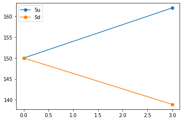
The Binomial Asset Pricing Model uses discrete time periods where the option can take one of two values (hence binomial). Let \(S_0\) be the intial price of the stock at \(t_0\). At time \(t_1\), the stock is expected to be at one of two prices,\(S_1(E_u) = uS_0\) or \(S_1(E_d) = dS_0\). Here \(E_u\) and \(E_d\) are the events for the price levels corresponding to multiplicative factors \(u\) and \(d\). We assume that \(0 < d < 1 < u\), further we assume, for simplicity, that \(d = \frac{1}{u}\). We can visualize this below for \(S_0=145\) and \(u=1.08\):

import matplotlib.pyplot as plt

s_u = [150,1.08*150]
s_d = [150,(1/1.08)*150]
plt.plot([0,3],s_u,'o-',label='Su')
plt.plot([0,3],s_d,'o-',label='Sd')
plt.legend()
plt.plot()
plt.show()

The probability of each event follow the binomial distribution, that is if \(P(E_u) = p\), then \(P(E_d)=1-p\). Now that we know the possible values of the underlying asset at \(t_1\), we can price the option in a way so that it is risk neutral. Risk neutral indicates that we don’t really care about the risk of an asset; we’re indifferent to the probability of a return or the probability of a loss. This implies that the value of our portfolio, which includes the option, needs to have the same value reguardless of whether \(E_u\) or \(E_d\) occurs. We can accomplish this by using a strategy known as delta hedging. Delta hedging involves creating a portfolio consisting of shares of the underlying stock, the option and cash invested in a market that earns at the risk free rate \(r\).

Suppose we think that the stock will decrease in value. In this case, we can take a short position in a call option; that is we sell call options with the value being the sale price of the option if the stock decreases. We can hedge against this by also purchasing shares of the stock in such a way as to offset the loss incurred if the stock price increases.

Let \(X_0\) be the intial wealth at time \(t_0\) and \(\Delta_0\) be the number of shares purchased at time \(t_0\). If \(f^x\), where \(x \in {u,d}\), is the value of the option at \(t_1\) then the wealth at \(t_0\) is given by

\[X_1^x = e^{rT}(X_0-\Delta_0S_0)+(\Delta_0S_1-f^x)\]

Note that we subtract the value of the option since we are shorting it. For our strategy to be risk neutral we need

\[X_1^u = X_1^d\] \[e^{rT}(X_0-\Delta_0S_0) + (\Delta_0S_0u-f^u) = e^{rT}(X_0-\Delta_0S_0) + (\Delta_0S_0d-f^u)\] \[\Delta_0S_0u-f^u = \Delta_0S_0d-f^d\] \[\Delta_0 = \frac{f^u - f^d}{S_0u-S_0d}\]

This implies the number of shares we want to purchase is related to the change in value of the option to the change in share price. Let’s use the option given previously, where it specifies a single share. Then since we are selling the option then the value of the option is as follows

\[f^u = 150-170 = 20 \text{ and } f^d = 0\]

Then

\[\Delta_0 = \frac{20-0}{170-140} = \frac{20}{30} = \frac{2}{3}\]

So the value of the portfolio is

\[X_1^u = e^{rT}(X_0-\frac{2}{3}(150)) + (\frac{2}{3}(170)-20) = e^{rT}(X_0-100)) + 93.33\]

or

\[X_1^d = e^{rT}(X_0-\frac{2}{3}(150)) + (\frac{2}{3}(140)-0) = e^{rT}(X_0-100)) + 93.33\]

To price the option, we now must find the present value of So for every share we sell a call option, we must buy 1.5 shares to hedge our position. Generally, we can’t buy 1.5 shares, and options contracts are sold for 100 shares, so really it’s 150 shares for an options contract.

So we have the number of shares we need to buy for each option we purchase to create a risk neutral portfolio. However, we still do not have a price we should pay for the option. We can find this from the idea that the present value of the portfolio should equal the cost of setting up the portfolio; that is

\[(\Delta_0S_0u - f^u)e^{-rT} = \Delta_0S_0 - f\]

where \(f\) if the option price at \(t_0\). From this then, it follows that

\[\Delta_0S_0 - f = (\Delta_0S_0u - f^u)e^{-rT}\] \[\implies f = S_0\Delta_0(1-ue^{-rT})+f^ue^{-rT}\]

Substituting in \(\Delta_0\) from earlier

\[f = S_0\frac{f^u - f^d}{S_0u-S_0d}(1-ue^{-rT})+f^ue^{-rT}\] \[f =\frac{f^u(1-ue^{-rT}) - f^d(1-ue^{-rT}) + f^ue^{-rT}(u-d)}{u-d}\] \[f = \frac{f^u-f^ude^{-rT} - f^d(1-ue^{-rT})}{u-d}\] \[f = \frac{f^u(1-de^{-rT}) + f^d(ue^{-rT}-1)}{u-d}\]

Setting

\[p = \frac{e^{rT} - d}{u-d}\]

It can be easily shown that

\[f = e^{-rT}[pf^u + (1-p)f^d]\]

We now have a price for the option at time \(t_0\) given that we want to use delta hedging to create a riskless portfolio.

Let’s check the price we find based on this equation to the bounds we found in the previous post using the stock above. Let’s also assume \(r=0.01\) and \(T=3\) months.

\[u = 1.08\text{, and } d = 0.926\]

So

\[p = \frac{e^{0.01*\frac{3}{12}} - 0.926}{1.08-0.926} = 0.496\]

We also have that

\[f^u = 162-145 = 17 \text{, and } f^d = 0\]

So the the price of the option should be

\[f = e^{-0.01*\frac{3}{12}}[17* 0.496+ (1-0.496)*0] = 8.41\]

We know from the previous post that a call option has bounds

\[\max(S_0-Ke^{-rT},0) \leq f \leq S_0\]

Clearly our price is less than the upper bound (current stock price). What about the lower bound?

\[S_0 - Ke^{-rT} = 150 - 145e^{-0.01*\frac{3}{12}} = 5.362\]