Fundamentals - Decision Trees

This post is the start of a series of posts I will make about some fundamental data science methods. I am making these to keep my knowledge of machine learning fundamentals strong and hopefully provide a nice/clear explanation of these methods. To start, I am going to talk about a type of model that is very powerful and very popular, the decision tree. I will follow this post with another post on ensemble methods and the ensembling of decision trees into random forests, a popular use of decision trees.

Introduction

Consider a classification problem with input space (feature space) \(\Omega\) and output space \(\omega\) along with a sample set \((X,Y) \subset (\Omega,\omega)\). Since this is a classification problem, \(\omega\) consists of a finite set of values, for example two \(\omega =\){ \(c_0,c_1 \)} (that is, binary classification). For the binary case, \(\omega\) defines a partition of the input space into two sets, \(\Omega = \Omega_{c_1}\cup \Omega_{c_2}\), where \(\Omega_{c_1}\) contains all objects classified as \(c_1\) and \(\Omega_{c_2}\) all object classified as \(c_2\). Given this, a classification model, \(\phi: \Omega \rightarrow \omega\) also defines a partition of \(\Omega\) as it approximates \(\Omega\) as some \(\Omega^\phi= \Omega_{c_1}^{\phi} \cup \Omega_{c_2}^{\phi}\). This approximation is based on an approximation of the output space \(Y\) as \(\hat{Y}\) using the input space sample\(X\). That is \(\phi(\vec{x})=\hat{y}\) for \(\vec{x} \in X\). This can be generalized to multiclass classification with \(\omega=\){\(c_1,c_2,c_3,…,c_n\)} by considering partitions for each class \(\Omega = \Omega_{c_1} \cup \Omega_{c_2} \cup…\cup \Omega_{c_n}\). Extension of this partition idea to regression, which has a continuous output space, is slightly trickier as one must find a way to take a single value from a partition and map to continuous output \(\omega\). We will discuss on this in the section on regression trees.

We now want to develop a method to partition our input space \(\Omega\) using the sample set \((X,Y)\) and a function \(\phi\) trained on \((X,Y)\), such that the partitioning of \(\Omega\) by \(\phi\) is as close to the true partition as possible. Decision tree, aka classification trees or regression, allow us to create such a partitioning.

Decision Trees

To start, we need a few definitions from graph theory.

Def 1: A tree is a graph \(G = (V,E)\) in which any two vertices are connected by exactly one path. That is, a graph with no cycles.

Def 2: A rooted tree is a tree in which a single vertex is designated as the root of the tree.

Def 3: If the exists an edge from a vertex \(v_1\) to a vertex \(v_2\), then \(v_2\) is said to be the child of \(v_1\) and \(v_1\) is the parent of \(v_2\). A vertex without any child vertices is a leaf vertex.

Def 4: A binary tree is a rooted tree where all non-leaf vertices have exactly two children.

A decision tree then is a model \(\phi:\Omega \rightarrow \omega\), that can be represented by a rooted tree. How does this represent a partition? What we will do is let each vertex in the tree represent some partition of \(\Omega\) and each edge represent some question that defines a partition rule of a parent partition. So we can see that child vertices are partitions of a parent vertex partition. The root vertex, which has no parent, is the entire input space \(\Omega\). Let’s take a look at an example.

Consider the following set with \(X \subset \Omega = [0,1]\times[0,1]\) and \(Y \subset \omega =\){\({red,blue}\)}

import numpy as np
import matplotlib.pyplot as plt

x1_red1 = np.random.uniform(0,1,15)
x1_red2 = np.random.uniform(0,0.5,10)
x2_red1 = np.random.uniform(0,0.5,15)
x2_red2 = np.random.uniform(0,1,10)
x1_blue = np.random.uniform(0.5,1,25)
x2_blue = np.random.uniform(0.5,1,25)

plt.scatter(x1_red1, x2_red1,color='r')
plt.scatter(x1_red2, x2_red2,color='r')
plt.scatter(x1_blue, x2_blue, color = 'b')
plt.xlabel('x_1')
plt.ylabel('x_2')
plt.show()

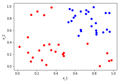
Now we want to partition this set based on questions we can ask about the space or partition. We start first by partitioning the entire space with the question is \(x_1\) less than or equal to 0.5? This question then splits the space into two partitions, those points with \(x_1 \leq 0.5\) and \(x_x > 0.5\). We can visualize this as

plt.scatter(x1_red1, x2_red1,color='r')
plt.scatter(x1_red2, x2_red2,color='r')
plt.scatter(x1_blue, x2_blue, color = 'b')
plt.plot((0.5, 0.5), (0, 1), 'k-')
plt.xlabel('x_1')
plt.ylabel('x_2')
plt.show()

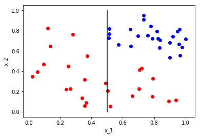
Let’s call these partitions \(\Omega_{x_1\leq 0.5}\) and \(\Omega_{x_1>0.5}\). Now that we’ve partitioned the whole space, we now want to ask a question that partitions one of the partitions. Since we are looking for partitions that will separate our class \({red,blue}\), we do not need to partition \(\Omega_{x_1\leq 0.5}\) as it contains only a single class. What is a question that we can ask to partition \(\Omega_{x_2>0.5}\)? How about is \(x_2\) greater than or equal to 0.5? This results in the following

plt.scatter(x1_red1, x2_red1,color='r')
plt.scatter(x1_red2, x2_red2,color='r')
plt.scatter(x1_blue, x2_blue, color = 'b')
plt.plot((0.5, 0.5), (0, 1), 'k-')
plt.plot((0.5,1),(0.5,0.5),'k-')
plt.xlabel('x_1')
plt.ylabel('x_2')
plt.show()

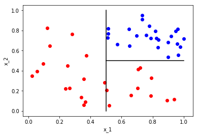
We now have three partitions that completely separate our classes; \(\Omega_{x_1\leq 0.5}\), \(\Omega_{(x_1 > 0.5, x_2 <0.5)}\) and \(\Omega_{(x_1>0.5, x_2\geq 0.5)}\). The class partitions can then be written as \(\Omega_{red} = \Omega_{x_1\leq 0.5} \cup \Omega_{(x_1 > 0.5, x_2 <0.5)}\) and \(\Omega_{blue} = \Omega_{(x_1>0.5, x_2\geq 0.5)}\). Note: this notation will get very clunky as the number of questions increases, but these questions form our function \(\phi\) as it were. So now, how might we represent this as a decision tree? Remember, each vertex represents a space/partition and each edge an answer to a question. The following is a tree representation of our example.

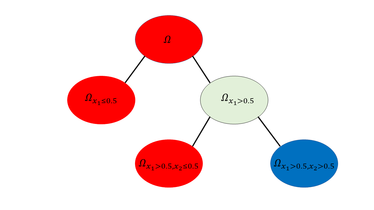
So we can see now that a decision tree is a representation of a set of questions and partitions. Now you may ask that while this is nice, the questions here were easy due to our knowledge of the data, what happens when we don’t know how the data (that is the sample) was created or the actual distribution the data comes from? We will get to that in a moment but first another pressing matter. Now that we have a model, if we were given a new sample or datapoint, how can we determine that class?

For example, suppose we were given \((0.8,0.3)\) and asked to determin whether this is red or blue. Well, we just ask the questions and follow the path down the tree! So for instance from the first questions, \(x_1=0.8\) is greater than 0.5 so this ends up in the \(\Omega_{x_1>0.5}\). Now we see if we can ask another question, which we can and since \(x_2=0.3\) is less than 0.5, the sample now ends up in the \(\Omega_{(x_1 > 0.5, x_2 <0.5)}\) partition. At this point we can no longer ask anymore questions (as this is a leaf vertex), but how do we label the point. We will discuss this further later, but for now we just let majority vote in the partition determine the label. In this case, all points in the partition are red so we label our new point red as well. And there you have, a bare bones discussion of decision trees and how they work. Now we will go into more detail. Note, we will primarily discuss binary decision trees which allow for yes/no questions only. It is possible to have non-binary splits, but we leave that for another post.

Splitting Vertices

Before getting into the process of developing questions and splitting vertices/partitions, let’s first define what it means for a question/split to be “good”. This requires us to define a loss function to determine how well the new partitions match the actual partitioning. Again, let us stay with the classification problem at the moment. If we label points in the partition represented by a vertex using majority vote, what is the loss (or sometimes called, the impurity)? We want a loss function that is minimized (that is, equal to zero) when all points belonging to the partition are of the same class and maximized when there is an equal amount of all classes in the partition (that is equally probability for each class for a randomly selected point). The former case being pure and the latter being maximally impure. What are some possible loss functions?

One possible loss function is classic entropy. This is the most popular loss function for classification problems using models such as logistic regression or neural networks. Entropy (called cross entropy for binary classification) is defined as follows:

def 5: Entropy \(S\) is given by

\[S = -\sum_i p_i\log{p_i}\]

Where \(p_i\) is the probability of the \(i\)th class in the partition.

We do not know the actual probability of each class but we can approximate it using \(p_i=\frac{|\Omega_i|}{|\Omega|}\) where \(\Omega\) is the partition under consideration, \(\Omega_i\) is the set of point corresponding to class \(i\) and || is the cardinality function. We can verify that this impurity measure is minimal when the partition is pure and maximal when each class has equal probability by plotting cross-entropy. Not that for two classes \(p_1=1-p_2\) and vice versa.

x = np.linspace(0.0001,.9999,100) #0.0001 and .9999 used to prevent log of zero
y = -(x*np.log(x)+(1-x)*np.log(1-x))

plt.plot(x,y)
plt.title('Cross entropy')
plt.show()

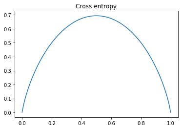
As this plot shows, cross-entropy reaches a maximum when \(p_1=p_2=0.5\) and is minimal then either \(p_1=0\) or \(p_2=0\) which is what we wanted.

However, entropy is not the only impurity measure. Another popular one is the Gini index.

Def 6: Gini index \(G\) is given by

\[G= 1-\sum_i (p_i)^2\]

Where again, \(p_i\) is the probability of class \(i\) in the partition. We can check that this also meets our requirements regarding minimal and maximal impurity.

x = np.linspace(0,1,100)
y = 1-x**2-(1-x)**2

plt.plot(x,y)
plt.title('Gini Index')
plt.show()

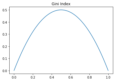
Indeed this does meet our requirements, though the maximal value is lower than that of entropy. Either of these measures is fine as they meet our requirements, though certain algorithms prefer one to the other. The CART algorithm uses Gini while C4.5 and ID3 use entropy. We will note in a moment that there are some differences in what type of split Gini and entropy prefer, but we first need to discuss choosing between splits.

So now we know how to measure how “good” a split or question is, can we use this to compare two split to determine which is better? We can define the impurity decrease as the difference between the current impurity (parent vertex) and the resulting impurity of the child vertices.

Def 7: Impurity decrease is given by

\[ID = S_P - \frac{|\Omega_{C_L}|}{|\Omega_P|}S_{C_L} - \frac{|\Omega_{C_R}|}{|\Omega_P|}S_{C_R}\]

for entropy and

\[ID = G_P - \frac{|\Omega_{C_L}|}{|\Omega_P|}G_{C_L} - \frac{|\Omega_{C_R}|}{|\Omega_P|}G_{C_R}\]

for Gini. Where \(\Omega_P\) is the set of points in the parent vertex and \(\Omega_{C_R}\) and \(\Omega_{C_L}\) are the set of points in the left and right child respectively.

We thus want to choose splits that maximize the impurity decrease. Note, for entropy, this is called the information gain due to it’s relations to information theory. You can think of a split as giving more information about the classes and that we want the split that maximizes this information.

Okay, so now we know how to determine if a question is better than another, how do we determine the set of questions? The questions will depend on the type of variable we are considering. Note that we will only ask questions of a single variable at a time (it is possible to partition on multiple variables, but rarely done). In general there are two types of variables; unordered and ordered. Unordered variables are categorical variables while ordered are continuous and ordinal. For categorical variables, we can only ask whether the variables is equal to a certain value. Therefore, for a categorical variable, the maximum number of questions we can ask (or splits we can make) is one minus the unique number of values the variable can take. For ordered variables, we can ask if the variable is less than or greater (or \(\leq\), \(\geq\)) than a given value (though these are essentially the same). For ordinal variables, the maximal number of splits is again one minus the unique number of possible values. For continuous though, the number of splits is infinite. Therefore we need a way to use the data at hand to determine a finite number of splits.

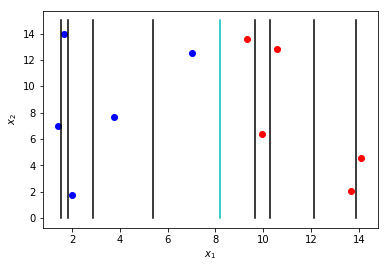
One way to handle continuous variables is to observe the unique number of values the data takes and have one minus that number. The actual split positions then are \(\frac{a-b}{2}\), where \(a\) and \(b\) are consecutive values that the variable can take. This can create a large number of possible splits considering each datapoint in the sample set may have a unique value for that variable. The figure below shows possible splits for the \(x_1\) variables. From this, we can clearly see the cyan colored split will give us the highest information gain.

x = np.random.uniform(1,15,10)
y = np.random.uniform(1,15,10)
c = np.sort(x)
plt.scatter(c[:5],y[:5],color='b')
plt.scatter(c[5:],y[5:],color='r')
for i in range(9):
    a = (c[i+1]+c[i])/2
    if i!=4:
        plt.plot((a,a),(0,15),'k')
    if i==4:
        plt.plot((a,a),(0,15),color='c')
plt.xlabel('$x_1$')
plt.ylabel('$x_2$')
plt.show()

A very nice result of selecting variables and splits based on a loss criteria is that it performs intrinsic feature selection. A feature (variable) where no split give much reduction in impurity will not be selected during model construction. We can therefore find important and irrelevant features based on their use within the model. Decision trees can actually be used as a feature selection tool prior to using other models such as logistic regression or neural networks.

Regression

The pervious discussion focused on classification, what about regression? For regression, we have continuous values for \(\omega\) rather than a discrete set of classes. We therefore can’t use the loss functions nor the labeling method defined in the previous section for regression so we’ll need regression specific measures. The loss function needs to give the difference between the model approximation value and the true value. We can use the popular loss function for regression, squared error

Def 8: Square error of an estimated regression value \(\hat{y}\) given the true value \(y\) is \(Err = (y-\hat{y})^2\)

Where \(\hat{y}\) is the model result. This loss function enhances the impact of large errors while reducing the impact of small errors. We also need to determine the value the decision tree provides at a leaf vertex. Since regression problems provide continuous value in the output space \(\omega\), we cannot have a majority vote (all \(y\) values in the leaf may be unique). We will instead use the average of all \(y\) values in the leaf as our model output. It can be shown the average minimized the square error loss, but I will leave that proof for the reader. To put formally

Def 9: Regression output for Decision Tree. Let \(X’,Y’)\subset (X,Y)\) be a partition on a leaf vertex and \(Y’ =\) {\( {y_1,y_2,…,y_{N}\)} and \(N = |(X’,Y’)|\). Then the output of the decision tree model at that leaf is given by \(\hat{y} = \frac{1}{N}\sum_{i=1}^N y_i\)

Now that we have a loss and model output functions, we can perform the same process as in classification trees. We look for splits what minimize the square error given the average of the resulting partition spaces as outputs.

Stopping

Now that we have methods to choose questions to ask and choose which split is the best, how do we know when to stop “growing” the tree? That is, when do stop spitting vertices? Splitting of decision trees can be continued until each point in the training set resides on a leaf vertex (or at least until the partition represented by the vertex is homogeneous with respect to a class) may be possible, though due to noise this is unlikely. Noise in the data can cause a vector \(\vec{x}\in X\) to have multiple class labels, in which case no partition can separate these labels. Suppose though that this is not the case and every point \(\vec{x}\in X\) has a unique label, then we can perfectly classify the training set with zero loss by partitioning until each \(\vec{}\) is in it’s own partition. However, this will significantly overfit the data, capturing all of the noise in the training set and have very poor results on data not within the training set. To prevent this overfitting, there are a few methods to determine when splitting of vertices should be stopped.

• Set a vertex as a leaf if it’s partition contains less than \(N_{min}\) samples
• Set a vertex as a leaf if it’s depth is greater or equal to a depth threshold \(d_{max}\)
• Set a vertex as a leaf is the total decrease in impurity (or square loss) is less than a fixed threshold \(\beta\)
• Set a vertex as a leaf is there is no split such that each resulting vertex (partition) both have at least \(N_{leaf}\) samples

The depth of a vertex is the number of parent vertices (or number of splits) above the one in consideration. Each of these methods help to prevent decision tree models from overfitting and capturing the noise. Let’s take a look at an example of how the max depth changes the output of a decision tree regression model. We use sklearn decision tree regressor for this.

from sklearn.tree import DecisionTreeRegressor

k=100
x = np.linspace(0,10,k).reshape(-1,1)
y = (x-4)**2+np.random.normal(0,2,k).reshape(-1,1)

dt1 = DecisionTreeRegressor(max_depth=3)
dt2 = DecisionTreeRegressor(max_depth=5)
dt1.fit(x,y)
x_f1 = dt1.predict(x)
dt2.fit(x,y)
x_f2 = dt2.predict(x)

plt.plot(x,y,'o',color='k')
plt.plot(x,x_f1,'y',label='$d_{max}$=3')
plt.plot(x,x_f2,'r',label='$d_{max}$=5')
plt.legend()
plt.show()

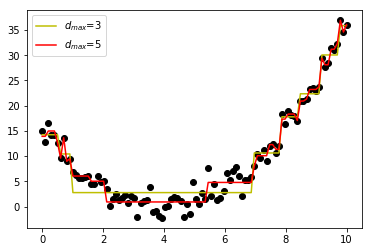
As we can see, restricting the depth of the model underfits the data (somewhat) while increasing the depth fits some of the noise (overfitting). Care must be taken when selecting stopping parameters to find the right balance between overfitting and underfitting the data.

Interpretability

One of the nicest features of decision trees is their ease of interpretability. If we want to know why a label was given to a certain point, we only need to follow the path of splits taken. For instance, in our first example, if we were given a point(0.8,0.4) to classify, the model would produce a class label of red. If we ask why, the answer would be because \(x_1\) is greater than \(0.5\) and \x_2\) is less than \(0.5\). For very complex models with lots of input features, this maybe be very cumbersome, but an explanation is still there. For certain areas of application, such as finance, explainable models are very important and thus, decision trees would be a great choice.

Conclusion

That concludes the discussion of Decision Trees. These models are very popular for many reasons

• Non-parametric; can model complex relationships between input and output without assumptions
• Can handle categorical and continuous data easily
• Intrinsic feature selection and are robust irrelevant features
• Robust to outliers or errors in data
• Easily interpretable

These are very powerful classification models due to their ability to partition space as opposed to create continuous, smooth decision boundaries which is what many classification methods. For regression, decision trees are very useful, but prone to overfit some noise, even when using stopping criteria (see above figure). We also see that using the average value in the partiton creates a flat, linear value within that partition which may resulting in high error. For highly nonlinear data, regression trees may need very relaxed stopping criteria resulting in a deep, inefficient complex model that another method may handle better. Thanks for reading!