Fundamentals - Simple Linear Regression

To continue the posts on fundamental machine learning methods, in this discussion, we will cover the workhorse of regression techniques, simple linear regression.

Introduction

Linear regression is a widely used parametric model for regression. This model assumes a linear relationship between in the input variables \(X\) and the output variable(s) \(Y\). We can, however, augment this assumption by transforming the input variables using basis function expansion or kernels in order to model non-linear data. The output \(Y\) is still assumed to be linear, just in response to the transformed variables rather than the original variables. We will discuss this further later in the post.

The linear relationship between input and output variables can be given as follows

Def 1: Linear Regression, let \(\bf{x}\in X\subset \mathbb{R}^{n+1}\) for \(n\) features and \(y(\bf{x})\in Y\subset \mathbb{R}^1\). Under the assumption of linear relationship between \(\bf{x}\) and \(y\)

\[y(\mathbf{x}) = w_0+w_1x_1+w_2x_2+...+w_nx_n=\mathbf{w}^T\mathbf{x}+\epsilon\]

where \(\bf{w}^T\bf{x}\) is the scalar product between the input \(\bf{x}\)\and the model parameters (the weight vector) \(\bf{w}\). Note that the vector \(\mathbf{x}=(1,x_1,x_2,…,x_n)\), where the 1 is for the \(w_0\) coefficient causing the \(n+1\) dimensions. The \(\epsilon\) term is the residual error between the model predictions and the data. If the data is not noisy and the relationship is perfectly linear, this term would be zero. However, this is pretty much never the case.

It is often assumed that the residual error follows a Gaussian (or normal) distribution. That is, if a variable follows a normal distribution then

\[\epsilon \sim \mathcal{N}(\epsilon|\mu,\sigma^2) = \frac{1}{\sqrt{2\pi\sigma^2}}\exp{-\frac{1}{2\sigma^2}(\epsilon-\mu)^2}\]

We can connect this residual to the linear regression model explicitly, we can express the model as

\[p(y|x,\theta) = \mathcal{N}(y|\mu(\vec{x}),\sigma^2)\]

Where \(\mu(\vec{x}) =\bf{w}^T\bf{x}\) and \(\sigma^2\) is the constant noise in the data. The parameters, \(\theta\), for our model then are \((\mathbf{w},\sigma^2)\).

Maximum Likelihood Estimation (Least Squares)

Now that we have the model defined and know what parameters are needed, given some input and output data, how do we determine the optimal parameters \(\theta\)? A very common way to estimate parameters in statistical models is the maximum likelihood estimate (MLE), defined by

\[\hat{\theta} = \text{argmax}_{\theta} \log{p(X|\theta)}\]

If we assume that the input data \(X\) is independent and identically distributed, then we can rewrite the logarithm as

\[\log{p(X|\theta)} = \sum_i \log{p(y_i|\mathbf{x}_i,\theta)}\]

This is called the log-likelihood, for which we want to find the parameters \(\theta\) that maximize it. It is common that, rather than maximizing the log-likelihood, we minimize the negative log-likelihood (NLL)

\[NLL(\theta) = -\sum_i \log{p(y_i|\mathbf{x}_i,\theta)}\]

This is done as many optimization software are designed to find the minima of function rather than the maxima. In the end, the \(\theta\) that minimizes the negative log-likelihood is of course, the same \(\theta\) that maximizes the log-likelihood.

We can substitute our linear regression model into the NLL function, and assuming \(N\) samples, we obtain

\[\begin{split} NLL(\theta) &= -\sum_{i=1}^N \log{\left [\frac{1}{\sqrt{2\pi\sigma^2}}\exp{\left (-\frac{1}{2\sigma^2}(y_i-\mathbf{w}^T\mathbf{x}_i)^2\right )}\right ]}\\ &=\sum_{i=1}^N\left [-\log{\left (\frac{1}{\sqrt{2\pi\sigma^2}}\right )}-\log{\exp{\left(-\frac{1}{2\sigma^2}(y_i-\mathbf{w}^T\mathbf{x}_i)^2\right)}}\right ]\\ &=\frac{N}{2}\log{2\pi\sigma^2} + \frac{1}{2\sigma^2}\sum_{i=1}^{N}(y_i-\mathbf{w}^T\mathbf{x}_i)^2 \end{split}\]

OLS Solution

We now want to find the \(\bf{w}\) that maximizes the MLE. Let us rewrite the \(NLL\) in terms of the whole dataset \(X\) and we can ignore the first term in the equation as it will have zero derivative.

\[NLL(\mathbf{w}) = \frac{1}{2\sigma^2}(Y-X\mathbf{w})^T(Y-X\mathbf{w}) = \frac{1}{\sigma^2}\left [\frac{1}{2}\mathbf{w}^T(X^TX)\mathbf{w}-\mathbf{w}^T(X^TY)\right ]\]

Taking the gradient of this with respect to \(\mathbf(w)\) we get

\[\nabla_\mathbf{w}NLL(\mathbf{w})=\frac{1}{\sigma^2}\left [X^TX\mathbf{w}-X^TY\right ]\]

Setting equal to zero we can eliminate the \(\sigma^2\) and get

\[X^TX\mathbf{w} = X^TY\]

From which we can get the ordinary least squares or OLS solution

\[\hat{\mathbf{w}} = (X^TX)^{-1}X^TY\]

Notice that this solution has an inverse of the \(X^TX\) matrix. This can cause a problem if any of the input variables/features are perfectly colinear or multicollinear as \(X^TX\) would be singular. It thus important to remove any collinearity or multicollinearity before fitting the model.

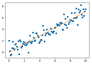
Let’s take a look at some simple examples using the OLS solution.

import numpy as np
import matplotlib.pyplot as plt

x = np.linspace(0,10,100)
y = 0.7*x+np.random.normal(0,0.8,100)

w = np.dot(np.dot(np.dot(x.T,x)**(-1),x),y)
plt.plot(x,y,'o')
plt.plot(x,w*x)
plt.show()
print('w:',w)

w: 0.704693458878835

From this we can see that the OLS solution is very close to our set weight; off by roughly 0.047. The plot of the fit also looks too be a good fit to the data. Thus, to summarize, the OLS solution provides a simple estimation of the \(\mathbf{w}\) parameters under the following assumptions we made explicitly:

• Linear relationship between \(X\) and \(Y\)
• Residuals follow a normal distribution with constant \(\sigma\)
• No multicollinearity

There are two other assumptions made with this solution we haven’t explicitly mentioned yet

• No correlation between any \(X\) and the error \(\epsilon\)
• No autocorrelation in the error \(\epsilon\)

These two are a result of assuming the variance of the model ((\ \sigma^2 \)) is fixed. If any of these assumptions are not met, then the OLS solution is not optimal or not possible. Therefore, it is important to check these assumptions prior to using the OLS solution as your estimate.

Conclusion

This was a basic discussion of the simplest form of linear regression and the OLS solution. In upcoming posts, we will continue the dscussion of linear regression with the basis function expansion, regularization techniques and stochastic gradient descent estimation of the \(\mathbf{w}\) parameters.